Forecasting Swiss ILI counts using simple log-normals by calendar week

options(digits = 4)  # for more compact numerical outputs
library("HIDDA.forecasting")
library("ggplot2")
source("setup.R", local = TRUE)  # define test periods (OWA, TEST)

In this vignette, we compute naive reference forecasts to be compared with the more sophisticated modelling approaches presented in the other vignettes. Our naive approach to predict weekly ILI counts from 2012-W48 to 2016-W51 (the OWA period) is to estimate a log-normal distribution from the counts observed in the previous years in the same calendar week. At each week, we estimate the two parameters using maximum likelihood as implemented in MASS::fitdistr().

The corresponding software reference is:

Ripley B (2023). MASS: Support Functions and Datasets for Venables and Ripley’s MASS. R package version 7.3-60, https://CRAN.R-project.org/package=MASS.

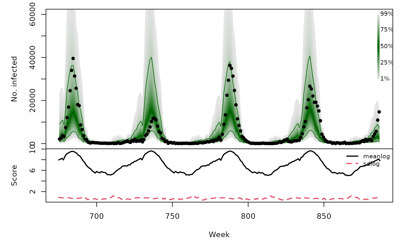
One-week-ahead forecasts

CHILI_calendarweek <- as.integer(strftime(index(CHILI), "%V"))
naiveowa <- t(sapply(X = OWA+1, FUN = function (week) {
    cw <- CHILI_calendarweek[week]
    index_cws <- which(CHILI_calendarweek == cw)
    index_prior_cws <- index_cws[index_cws < week]
    MASS::fitdistr(CHILI[index_prior_cws], "lognormal")$estimate
}))

.PIT <- plnorm(CHILI[OWA+1], meanlog = naiveowa[,"meanlog"], sdlog = naiveowa[,"sdlog"])
hist(.PIT, breaks = seq(0, 1, 0.1), freq = FALSE, main = "", xlab = "PIT")
abline(h = 1, lty = 2, col = "grey")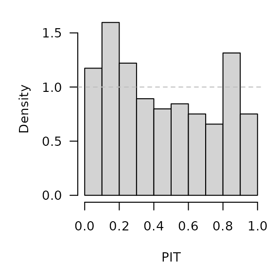

naiveowa_scores <- scores_lnorm(
    x = CHILI[OWA+1],
    meanlog = naiveowa[,"meanlog"], sdlog = naiveowa[,"sdlog"],
    which = c("dss", "logs"))
summary(naiveowa_scores)

##       dss            logs      
##  Min.   :10.4   Min.   : 5.43  
##  1st Qu.:12.2   1st Qu.: 6.48  
##  Median :13.9   Median : 7.82  
##  Mean   :14.9   Mean   : 8.06  
##  3rd Qu.:17.3   3rd Qu.: 9.40  
##  Max.   :27.6   Max.   :12.71

Note that discretized forecast distributions yield almost identical scores (essentially due to the large counts):

naiveowa_scores_discretized <- scores_lnorm_discrete(
    x = CHILI[OWA+1],
    meanlog = naiveowa[,"meanlog"], sdlog = naiveowa[,"sdlog"],
    which = c("dss", "logs"))
summary(naiveowa_scores_discretized)

##       dss            logs      
##  Min.   :10.4   Min.   : 5.43  
##  1st Qu.:12.2   1st Qu.: 6.48  
##  Median :13.9   Median : 7.82  
##  Mean   :14.9   Mean   : 8.06  
##  3rd Qu.:17.3   3rd Qu.: 9.40  
##  Max.   :27.6   Max.   :12.71

naiveowa_quantiles <- sapply(X = 1:99/100, FUN = qlnorm,
                             meanlog = naiveowa[,"meanlog"],
                             sdlog = naiveowa[,"sdlog"])
osaplot(
    quantiles = naiveowa_quantiles, probs = 1:99/100,
    observed = CHILI[OWA+1], scores = naiveowa,
    start = OWA[1]+1, xlab = "Week", ylim = c(0,60000),
    fan.args = list(ln = c(0.1,0.9), rlab = NULL)
)

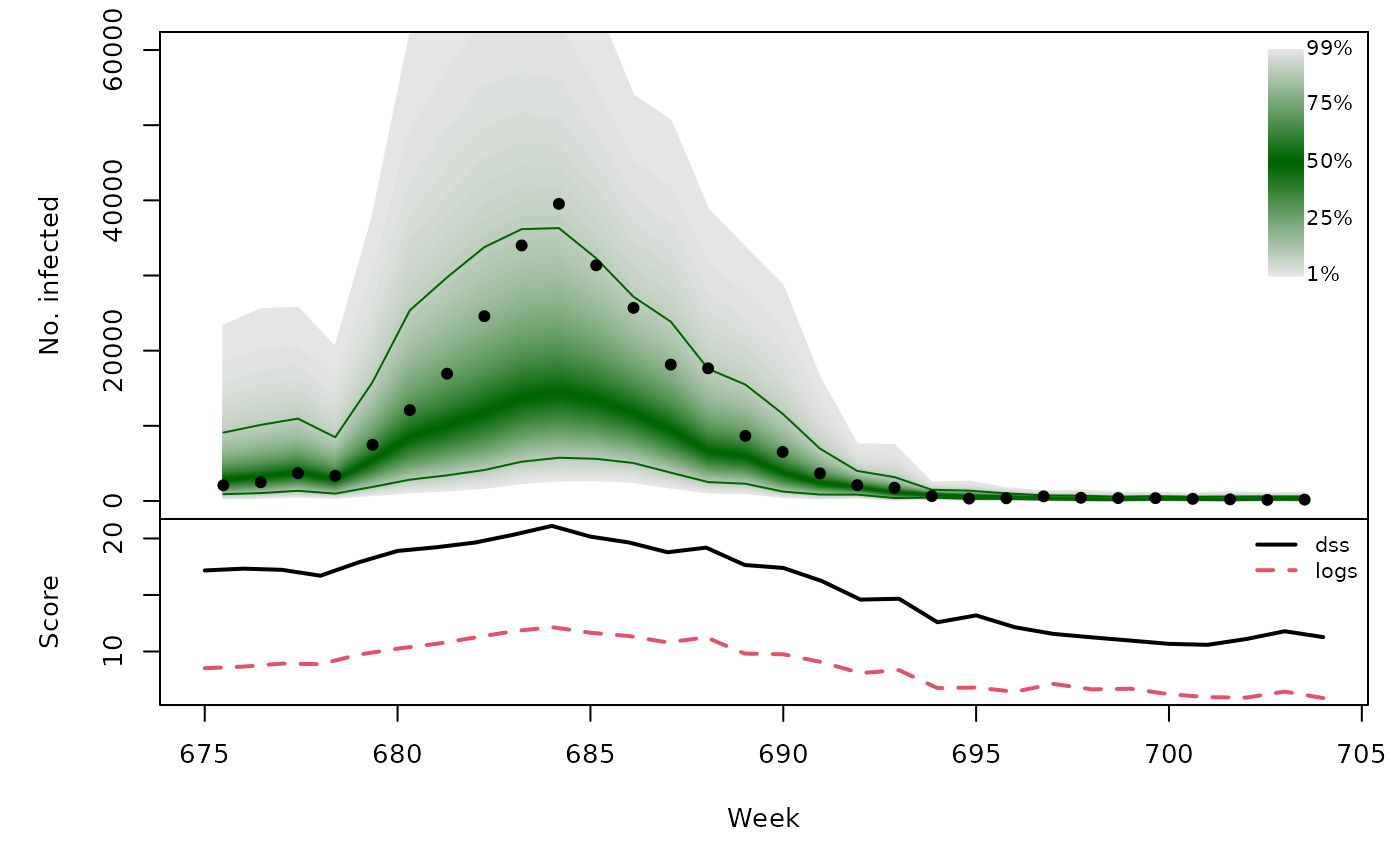
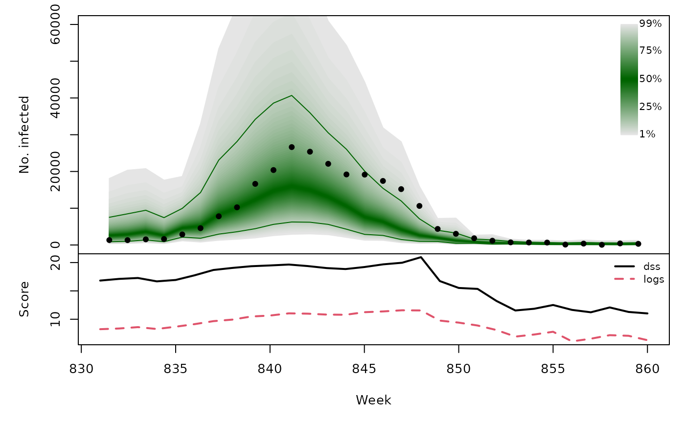
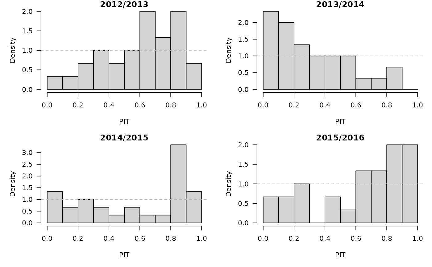
Long-term forecasts

With this naive forecasting approach, the long-term forecast for a whole season is simply composed of the sequential one-week-ahead forecasts during that season.

rownames(naiveowa) <- OWA+1
naivefor <- lapply(TEST, function (testperiod) {
    owas <- naiveowa[as.character(testperiod),,drop=FALSE]
    list(testperiod = testperiod,
         observed = as.vector(CHILI[testperiod]),
         meanlog = owas[,"meanlog"], sdlog = owas[,"sdlog"])
})

invisible(lapply(naivefor, function (x) {
    PIT <- plnorm(x$observed, meanlog = x$meanlog, sdlog = x$sdlog)
    hist(PIT, breaks = seq(0, 1, 0.1), freq = FALSE,
         main = format_period(x$testperiod, fmt = "%Y", collapse = "/"))
    abline(h = 1, lty = 2, col = "grey")
}))

t(sapply(naivefor, function (x) {
    quantiles <- sapply(X = 1:99/100, FUN = qlnorm,
                        meanlog = x$meanlog, sdlog = x$sdlog)
    scores <- scores_lnorm(x = x$observed,
                           meanlog = x$meanlog, sdlog = x$sdlog,
                           which = c("dss", "logs"))
    osaplot(quantiles = quantiles, probs = 1:99/100,
            observed = x$observed, scores = scores,
            start = x$testperiod[1], xlab = "Week", ylim = c(0,60000),
            fan.args = list(ln = c(0.1,0.9), rlab = NULL))
    colMeans(scores)
}))

##        dss  logs
## [1,] 15.70 8.729
## [2,] 15.81 8.499
## [3,] 16.12 9.114
## [4,] 16.33 9.095

Sebastian Meyer

2023-11-29

One-week-ahead forecasts

Long-term forecasts