Forecasting Swiss ILI counts using `kcde::kcde`
Sebastian Meyer
2026-07-02
Source:vignettes/extra/CHILI_kcde.Rmd
CHILI_kcde.RmdIn this vignette, we use forecasting methods provided by:
The corresponding software reference is:Ray E (2017). kcde: Kernel conditional density estimation with flexible kernel specifications. R package version 0.0.0.9000, commit 6f8c8e5c82ec63e2e8f8bc2a143ec75460d86ab4, https://github.com/reichlab/kcde/tree/6f8c8e5c82ec63e2e8f8bc2a143ec75460d86ab4.
Modelling
Note: we use a log-transformation of the CHILI counts in kcde.
Configuring kcde() is quiet lengthy and not shown here
(see the vignette sources for details).
We used 3 cores in parallel. Fitting the full bandwidth KCDE would take several days, so we used the diagonal bandwidth parametrization.
kcdefit$runtime / 60## user system elapsed
## 12.6609 0.4385 4.5948Unfortunately, the estimation function kcde() just
returns a list without a dedicated class. It is unclear to me how to
summarize the model fit or extract fitted values …
One-week-ahead forecasts
We compute 213 one-week-ahead forecasts from 2012-W48 to 2016-W51
(the OWA period).
The code is again lengthy and not shown here (see the sources for details).
Computing the 213 forecasts took 4.4 minutes (single core).
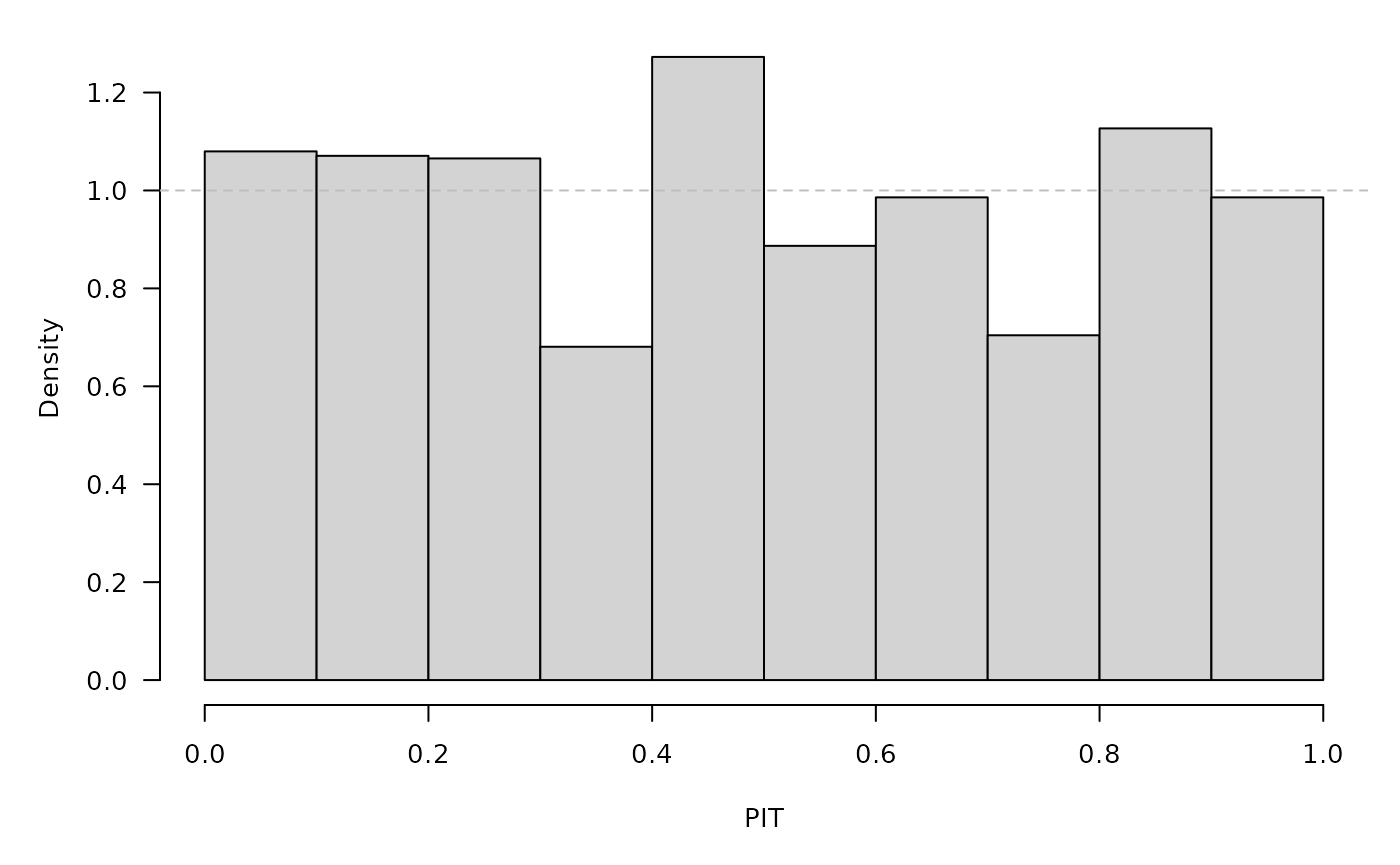
The PIT histogram is based on the pointwise ECDF of the samples from the predictive distributions.
##       DSS          log_score           AE
##  Min.   : 8.61   Min.   : 4.51   Min.   :    1
##  1st Qu.:11.02   1st Qu.: 6.52   1st Qu.:   99
##  Median :13.27   Median : 7.64   Median :  340
##  Mean   :13.79   Mean   : 7.80   Mean   :  956
##  3rd Qu.:16.85   3rd Qu.: 9.09   3rd Qu.:  910
##  Max.   :23.36   Max.   :13.01   Max.   :10872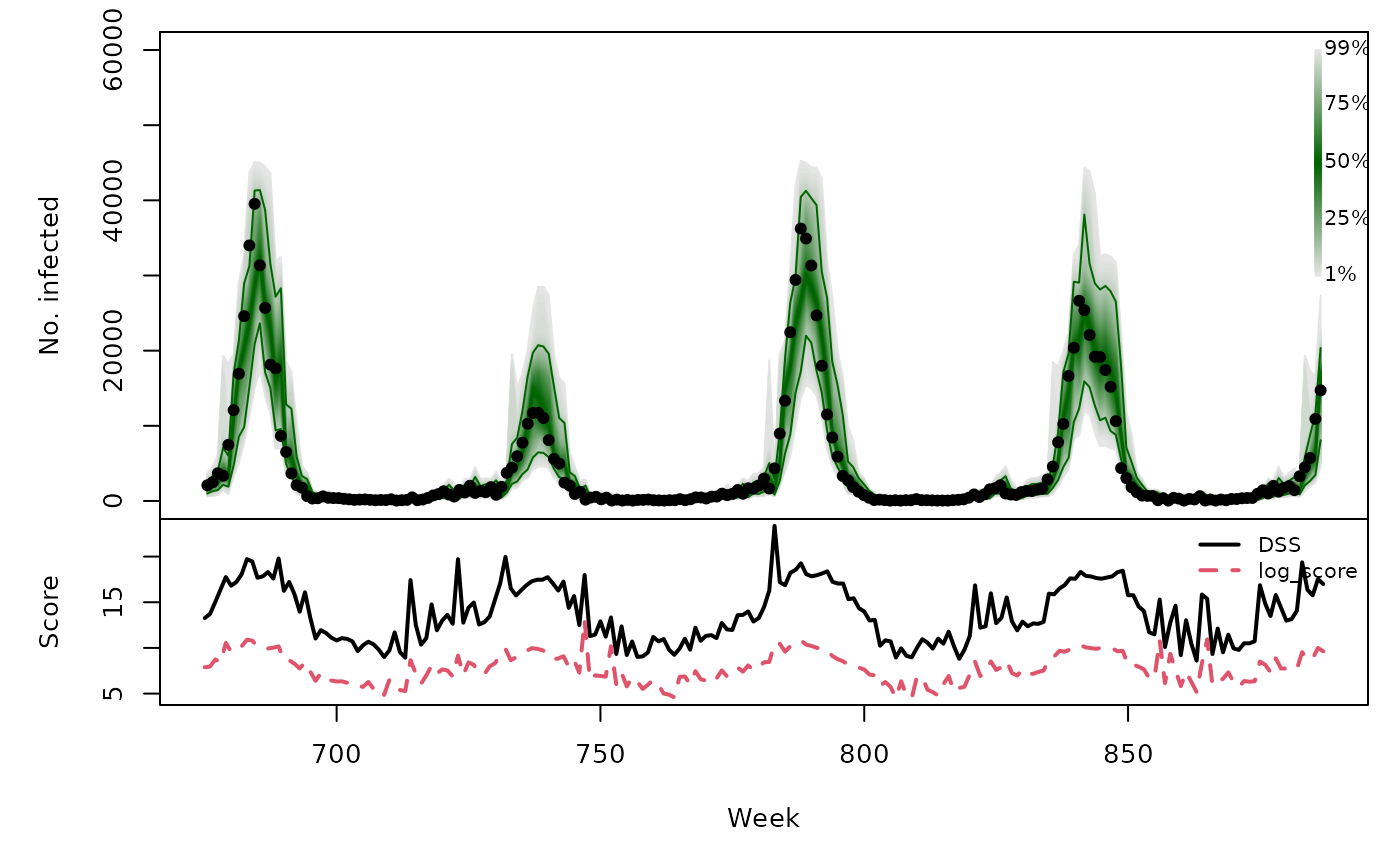
Long-term forecasts
We would need to rerun kcde() and subsequent predictions
for each of the three different training periods with
prediction_horizon varying from 1 to 30. Based on the
runtime of the above computations for a single training period and
prediction horizon, computing all long-term forecasts is estimated to
take approximately 13.5 hours. This is far beyond the runtimes of the
alternative prediction approaches, so we skip long-term forecasts with
kcde.