hhh4-Based Forecast Distributions

The function dhhh4sims constructs a (non-vectorized) probability mass function from the result of surveillance::simulate.hhh4() (and the corresponding model), as a function of the time point within the simulation period. The distribution at each time point is obtained as a mixture of negative binomial (or Poisson) distributions based on the samples from the previous time point.

dhhh4sims(sims, model)

Arguments

sims

a "hhh4sims" object from surveillance::simulate.hhh4().

model

the "hhh4" object underlying sims.

Value

a function(x, tp = 1, log = FALSE), which takes a vector of model$nUnit counts and calculates the (log-)probability of observing these counts (given the model) at the tp'th time point of the simulation period (index or character string matching rownames(sims)).

See also

logs_hhh4sims() where this function is used.

Author

Sebastian Meyer

Examples

library("surveillance")
#> Loading required package: sp
#> Loading required package: xtable
#> This is surveillance 1.22.1; see ‘package?surveillance’ or
#> https://surveillance.R-Forge.R-project.org/ for an overview.
CHILI.sts <- sts(observed = CHILI,
                 epoch = as.integer(index(CHILI)), epochAsDate = TRUE)

## fit a simple hhh4 model
(f1 <- addSeason2formula(~ 1, period = 365.2425))
#> ~1 + sin(2 * pi * t/365.2425) + cos(2 * pi * t/365.2425)
fit <- hhh4(
    stsObj = CHILI.sts,
    control = list(ar = list(f = f1), end = list(f = f1), family = "NegBin1")
)

## simulate the last four weeks (only 200 runs, for speed)
sims <- simulate(fit, nsim = 200, seed = 1, subset = 884:nrow(CHILI.sts),
                 y.start = observed(CHILI.sts)[883,])
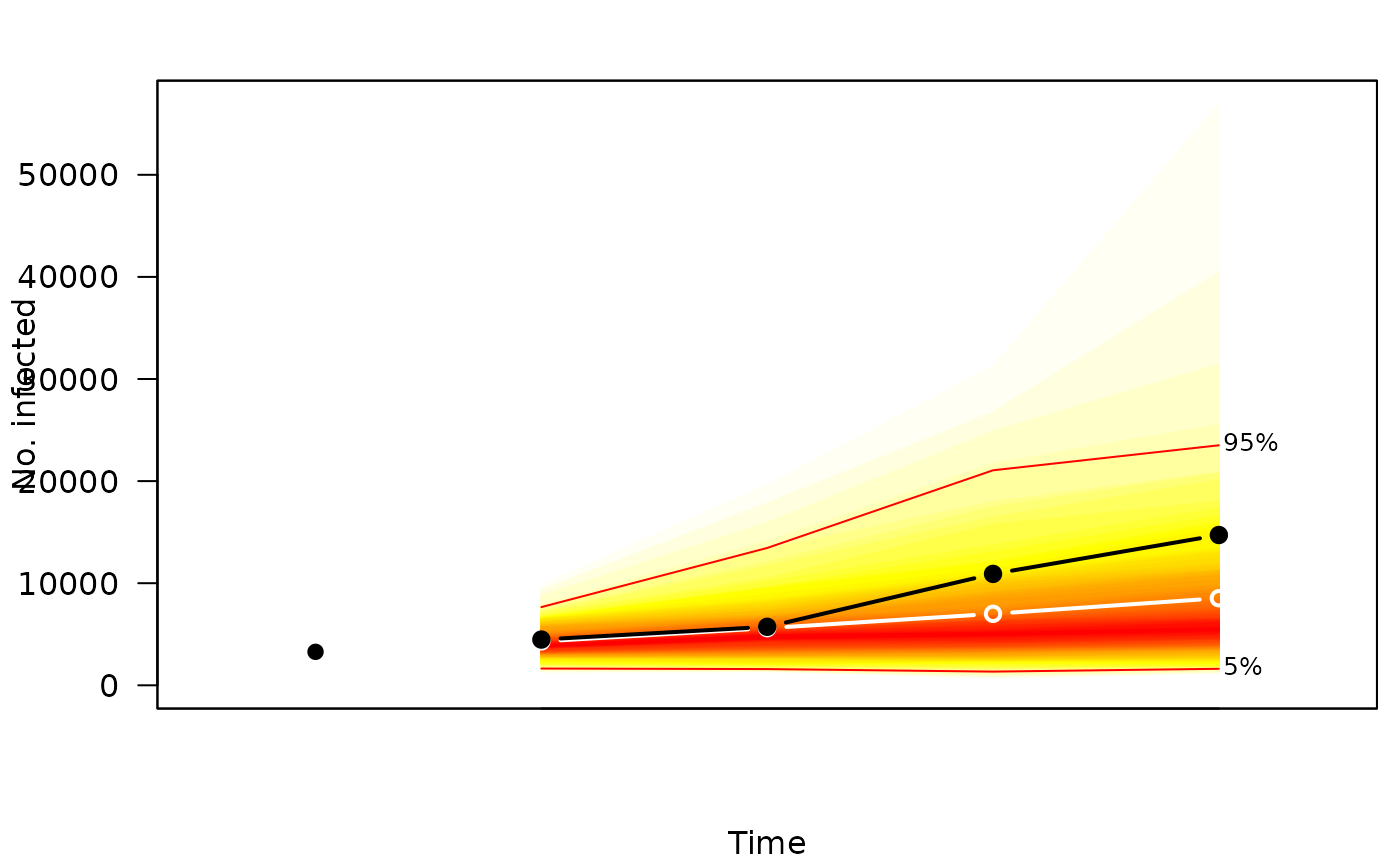
if (requireNamespace("fanplot")) {
    plot(sims, "fan", fan.args = list(ln = c(5,95)/100),
         observed.args = list(pch = 19), means.args = list(type = "b"))
}
#> Loading required namespace: fanplot


## derive the weekly forecast distributions
dfun <- dhhh4sims(sims, fit)
dfun(4000, tp = 1)
#> [1] 0.0002194578
dfun(4000, tp = 4)
#> [1] 0.0001069622
curve(sapply(x, dfun, tp = 4), 0, 30000, type = "h",
      main = "4-weeks-ahead forecast",
      xlab = "No. infected", ylab = "Probability")


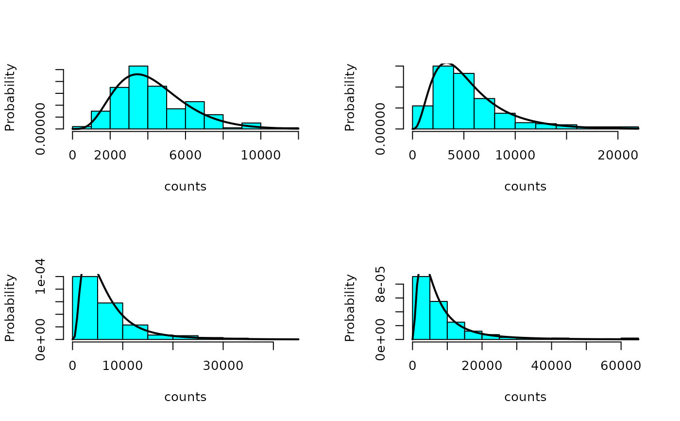
## compare the forecast distributions with the simulated counts
par(mfrow = n2mfrow(nrow(sims)))
for (tp in 1:nrow(sims)) {
    MASS::truehist(sims[tp,,], xlab = "counts", ylab = "Probability")
    curve(sapply(x, dfun, tp = tp), add = TRUE, lwd = 2)
}


# \dontshow{
## verify distribution at the first time point (i.e., one-step-ahead NegBin)
stopifnot(identical(
    sapply(0:100, dfun, tp = 1),
    dnbinom(0:100,
            mu = meanHHH(fit$coefficients, terms(fit), subset = 884, total.only = TRUE),
            size = sizeHHH(fit$coefficients, terms(fit), subset = 884))
))
## check that we have a probability distribution at the last time point
.xgrid <- seq(0, 100000, by = 500)
stopifnot(abs(1 -
    integrate(approxfun(.xgrid, sapply(.xgrid, dfun, tp = 4)), 0, 100000)$value
) < 0.001)
# }